DAA Question Bank 2079

Explain the divide and conquer strategy for problem solving. Describe the worst-case linear time selection algorithm and analyze its complexity.

The divide-and-conquer strategy is a problem-solving approach that breaks down a complex problem into smaller, more manageable subproblems. These subproblems are then solved recursively, and their solutions are combined to solve the original problem. This strategy is often used in computer science to design efficient algorithms.

Three steps of the divide-and-conquer strategy:

1. Divide: Break the problem into smaller subproblems.
2. Conquer: Solve the subproblems recursively.
3. Combine: Combine the solutions to the subproblems to solve the original problem.

The divide-and-conquer strategy is an effective way to solve problems that have the following properties:

• The problem can be broken down into smaller subproblems of the same type.
• The subproblems can be solved independently of each other.
• The solutions to the subproblems can be combined to solve the original problem.

The divide-and-conquer strategy is often used to design algorithms for sorting, searching, and multiplying large numbers.

Worst-Case Linear Time Selection Algorithm

The worst-case linear time selection algorithm is a simple algorithm for selecting the kth smallest element in an unsorted array. The algorithm works by first partitioning the array into two subarrays of equal size, such that all elements in the first subarray are less than or equal to all elements in the second subarray. The algorithm then recursively selects the kth smallest element in the subarray that contains the kth smallest element of the original array.

The worst-case time complexity of the worst-case linear time selection algorithm is O(n), where n is the number of elements in the array. This is because the algorithm always takes n steps to partition the array, regardless of the input.

Analysis of Complexity

The time complexity of an algorithm is a measure of how long it takes the algorithm to run as a function of the size of its input. The time complexity of an algorithm is typically expressed using Big O notation, which describes the upper bound of the algorithm’s running time as a function of the input size.

The time complexity of the worst-case linear time selection algorithm is O(n), where n is the number of elements in the array that means that the algorithm will always take at most O(n) steps to complete, regardless of the input.

The worst-case linear time selection algorithm is an example of an algorithm with a linear time complexity that means that the algorithm’s running time increases linearly with the size of its input.

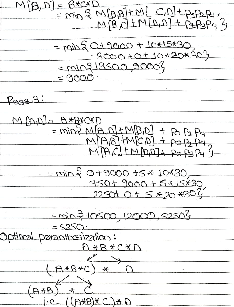
What do you mean by Backtracking? Explain the backtracking algorithm for solving 0-1
knapsack problem and find the solution for the problem given below:

Backtracking is an algorithm design technique that systematically explores a set of potential solutions to a problem, by trying to build a solution step by step, and backtracking (undoing or retracing steps) whenever it finds that a partial solution is not promising.

2nd part:

Backtracking algorithm for solving 0-1 knapsack problem:

1.start

2.Sort the items by value per weight.

3.Initialize the current solution to the empty set.

4.Recursively explore the space of possible solutions.

a. Add the current item to the current solution.

b. Check if the current solution is still feasible.

c. Check if the current solution is better than the best solution found so far.

d. Recursively explore the rest of the space of possible solutions.

e. Remove the current item from the current solution.

5.The best solution found so far is the solution to the 0-1 knapsack problem.

3rd part:

1. Sort the items by value per weight. This gives us the following sorted list:

Explain the iterative algorithm to find the GCD of given two numbers and analyze its complexity.

Algorithm to find GCD

1. Start
2. Read any two number say ‘m’ and ‘n’
3. If n==0, return the value of m as answer and stop
4. If m==0, return the value of n as answer and stop
5. Divide m by n and assign the remainder to r
6. Assign the value of m to n and n to r
7. stop

Analysis:

Time complexity: O(n)

Space complexity: O(1)

Generate the prefix code for the string ” CYBER CRIME” using Huffman algorithm and find the total number of bits required.

Define tractable and intractable problem. Illustrate vertex cover problem with an example.

Tractable problem

Tractable problem is a problem that can be solved efficiently using a known algorithm. The running time of a tractable algorithm is typically polynomial in the size of the input. For example, the shortest path problem is a tractable problem because it can be solved in polynomial time using Dijkstra’s algorithm.

Intractable problem

An intractable problem, also known as an NP-hard problem, is a problem that is believed to not have a polynomial-time algorithm. This means that the running time of the best known algorithm for an intractable problem is exponential in the size of the input. For example, the satisfiability problem (SAT) is an intractable problem because there is no known polynomial-time algorithm for solving it.

The vertex cover problem is an example of an intractable problem. Given an undirected graph G, a vertex cover of G is a subset of vertices in G such that every edge in G has at least one endpoint in the subset. The vertex cover problem is NP-hard, which means that there is no known polynomial-time algorithm for solving it in general.

Here is an example of the vertex cover problem:

A---B
|   |
C---D

In this graph, a vertex cover is {A, C}. This is because every edge in the graph has at least one endpoint in {A, C}.

Write short notes on:
a) Best, Worst and average case complexity

b) Greedy Strategy

a) Best-case complexity :  Best case time complexity refers to the minimum number of operation an algorithm needs to perform for the specific input. It is the most favourable situation for algorithm execution.

Worst-case complexity : Worst case time complexity refers to the maximum number of operation an algorithm needs to perform for the specific input. It is the least favourable situation for algorithm execution.

Average-case complexity : The average-case complexity of an algorithm represents the average amount of resources it requires to run over all possible inputs. It takes into account the frequency of different input scenarios to provide a more realistic estimate of the algorithm’s performance.

b)Greedy Strategy

Greedy strategy is a heuristic algorithm design technique that makes a locally optimal choice at each step of the algorithm, hoping that these choices will lead to a globally optimal solution. Greedy algorithms are often simple to implement and can perform well in practice, but they may not always find the optimal solution.

Greedy algorithms are particularly useful for problems with overlapping subproblems, where the optimal solution for a subproblem can be directly incorporated into the optimal solution for a larger problem. For example, the Huffman algorithm, which is used to create efficient prefix codes, is a greedy algorithm.

Trace the quick sort algorithm for sorting the array A[ ]={15,7,6,23, 18,34,25} and write it’s best and worst complexity.

The best-case complexity of quicksort is O(n log n). This occurs when the pivot element always divides the array into two roughly equal subarrays. In this case, the algorithm makes only log n recursive calls, and each recursive call performs a constant amount of work.

The worst-case complexity of quicksort is O(n^2). This occurs when the pivot element is always the smallest or largest element in the subarray. In this case, the algorithm makes n recursive calls, and each recursive call performs O(n) work.

Therefore, quicksort is an efficient algorithm for sorting arrays in general, but its worst-case performance can be quadratic.

Solve the following recurrence relations using masters method

a. T(n) = 2T(n/4) + kn², n > 1

=1 ,  n=1

b. T(n) = 5T(n/4) + kn , n > 1

=1  ,   n=1

 

 

Solve the following linear congrvences using Chinese Remainder Theorem.
X=l (MOD 2)
X=3 (MOD 5)
x=6 (MOD 7)

Find the edit distance between the string ” ARTIFICIAL” and “NATURAL” Using dynamic programming.

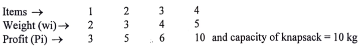
Find the MST from following graph using Kruskal’s algorithm.

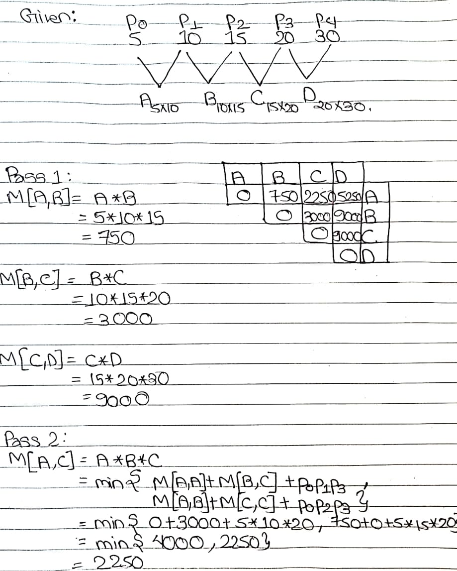
Write the dynamic programming algorithm for matrix chain multiplication. Find the optimal parenthesization for the matrix chain product ABCD with size of each is given as A_5×10 , B_10×15 , C_15×20 , D_20×30

The dynamic programming algorithm for matrix chain multiplication is a method for finding the minimum number of scalar multiplications required to multiply a chain of matrices. The algorithm works by building a table that stores the minimum number of scalar multiplications required to multiply all possible sub chains of the given chain.

Algorithm for dynamic programming algorithm for matrix chain multiplication.

1.start

2.Create a table M of size (n+1) x (n+1), where n is the number of matrices and fill the diagonal of the table with 0s.

3.For each subproblem (i, j), where 1 ≤ i ≤ j ≤ n, calculate the minimum number of scalar multiplications required to multiply matrices A_i, A_{i+1}, …, A_j using the following formula:

M[i , j] = min{M[i , k] + M[k+1, j] + p_i *p_{k+1} *p_j}

4.Once the table is filled, the optimal parenthesization can be found by tracing back through the table.

5.stop

2nd pard

To find the optimal parenthesization for the matrix chain product ABCD with given sizes, you can use dynamic programming to minimize the number of scalar multiplications. The goal is to find the optimal way to parenthesize the matrices to minimize the overall cost.

Let’s denote the matrices as follows:

• A: 5×10
• B: 10×15
• C: 15×20
• D: 20×30