DAA Question Bank 2078

Tribhuvan University

Institute of Science and Technology

2078

Bachelor Level / fifth-semester / Science

Computer Science and Information Technology( CSC314 )

Design and Analysis of Algorithms

Full Marks: 60 + 20 + 20

Pass Marks: 24 + 8 + 8

Time: 3 Hours

Candidates are required to give their answers in their own words as far as practicable.

The figures in the margin indicate full marks.

What are the elementary properties of algorithm? Explain. Why do you need algorithm? Discuss about analysis of the RAM model for analysis of algorithm with suitable example.

Algorithm is a step-by-step procedure, which defines a set of instructions to be executed in a certain order to get the desired output. Algorithms are generally created independent of underlying languages, i.e. an algorithm can be implemented in more than one programming language.

Characteristics of an Algorithm

• Unambiguous − Algorithm should be clear and unambiguous. Each of its steps (or phases), and their inputs/outputs should be clear and must lead to only one meaning.
• Input − An algorithm should have 0 or more well-defined inputs.
• Output − An algorithm should have 1 or more well-defined outputs, and should match the desired output.
• Finiteness − Algorithms must terminate after a finite number of steps.
• Feasibility − Should be feasible with the available resources.
• Independent − An algorithm should have step-by-step directions, which should be independent of any programming code.

We need algorithm because:

Algorithms play a crucial role in computer science. The best algorithm ensures that the computer completes the task in the most efficient manner. When it comes to efficiency, a good algorithm is really essential. An algorithm is extremely important for optimizing a computer program.

 

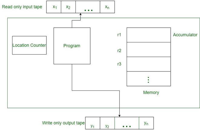
Random Access Machine (RAM)

Random Access Machine or RAM model is a CPU. It is a potentially unbound bank of memory cells, each of which can contain an arbitrary number or character. Memory cells are numbered and it takes time to access any cell in memory or say all operations (read/write from memory, standard arithmetic, and Boolean operations) take a unit of time. RAM is a standard theoretical model of computation (infinite memory and equal access cost). The Random Access Machine model is critical to the success of the computer industry.

Some key assumption to be made during analysis are :

1. For deceleration part time complexity will be O(1).
2. Basic arithmetic operations (addition, subtraction, multiplication, division) and logical operations (AND, OR, NOT) take constant time $O(1)$.
3. In cases of any loop time complexity will be O(n).
4. In case of nested loops time complexity will be O(1) x O(1) i.e O(n²).
5. If total memory refrences used by the algorithm is constant then space complexity will be O(1).
6. In case of array with n memory space space complexity will be O(n).

Example:

factorial(n)
{ 
   int i, fact =1;
   for(i=1; i<=n; i++)
     {
        fact = fact * i;
     }
   return fact;
}

for above algorithm  we see,

1. Declaration part have time complexity as O(1).
2. In loop :
   a.   i =  1 will have time complexity O(1).
   b.   i <= n will run the loop n times so it will have time complexity O(n).
   c.  i ++ is an arithmetic calculation so time complexity will be O(1).
3. return part will have time complexity as O(1).

finally time complexity will be : O(1)+O(1)+O(n)+O(1)+O(1) = 5O(1) + O(n) = O(n).

As space considered are constant so space complexity will be O(1).

 

Explain about the divide and conquer paradigm for algorithm design with suitable example. Write the Quick sort algorithm using randomized approach and explain its time complexity.

In the divide and conquer approach, a problem is divided into smaller problems, then the smaller problems are solved independently, and finally, the solutions of smaller problems are combined into a solution for the large problem.

Generally, divide-and-conquer algorithms have three parts −

• Divide the problem into a number of sub-problems that are smaller instances of the same problem.
• Conquer the sub-problems by solving them recursively. If they are small enough, solve the sub-problems as base cases.
• Combine the solutions to the sub-problems into the solution for the original problem.

Example:

A classic example of Divide and Conquer is Merge Sort. In Merge Sort, we divide the array into two halves, sort the two halves recursively, and then merge the sorted halves.

Randomized Quick Sort:

Randomized quick sort is called randomized if its behavior depends on input as well as the random value generated by the random number generator. The beauty of the randomized algorithm is that no particular input can produce worst-case behavior.

Algorithm:

RandQuickSort(A, l, r){
    if( l < r ){
        m = RandPartition(A, l, r);
        RandQuickSort(A, l, m-1);
        RandQuickSort(A, m+1, r);
    }
}

RandPartition(A, l, r){
    k = random(l, r);
    swap(A[l], A[k]);
    return Partition(A, l, r);
}

Partition(A, l, r){
    x = l;
    y = r;
    p = A[l];

    while(x < y){
        do{
            x++;
        }while(A[x] <= p);

        do{
            y--;
        }while(A[y] >= p);

        if( x < y ){
            swap(A[x], A[y]);
        }
    }

    A[l] = A[y];
    A[y] = p;

    return y;
}

Time Complexity:

• For the Wrost case, Time complexity is O(n²)
• For Best case, Time complexity is O(n log n)
• For Average case, Time complexity is O(n log n)

Explain in brief about the Dynamic Programming Approach for algorithm design. How it differs with recursion? Explain the algorithm for solving the 0/1 Knapsack problem using the dynamic programming approach and explain its complexity.

The dynamic programming approach is similar to divide and conquer in breaking down the problem into smaller and yet smaller possible sub-problems. But unlike, divide and conquer, these sub-problems are not solved independently. Rather, the results of these smaller sub-problems are remembered and used for similar or overlapping sub-problems.

Dynamic programming is used where we have problems, which can be divided into similar sub-problems so that their results can be re-used. Mostly, these algorithms are used for optimization. Before solving the in-hand sub-problem, the dynamic algorithm will try to examine the results of the previously solved sub-problems. The solutions of sub-problems are combined in order to achieve the best solution.

Characteristics:

Dynamic Programming works when a problem has the following features:

• Optimal Structure: If an optimal solution contains optimal visit solutions then a problem exhibits optimal substructure.
• Overlapping sub-problems: When a recursive algorithm would visit the same sub-problems repeatedly, then a problem has overlapping sub-problems.

If the problem has an optimal substructure, then we can recursively define an optimal solution. If a problem has overlapping sub-problems, then we can improve on implementation by computing each sub-problem only once.

Difference Between Dynamic Programming && Recursion:

With respect to iteration, recursion has the following advantages and disadvantages:

• Simplicity: often a recursive algorithm is simple and elegant compared to an iterative algorithm
• Space-inefficiency: every recursive call adds a layer to the system’s call stack. If the number of stacked recursive calls gets too large, the result is a stack overflow.

Every recursive algorithm can be implemented iteratively.

0/1 Knapsack Problem:

The 0/1 knapsack problem means that the items are either complete or no items are filled in a knapsack. For example, we have two items having weights of 2kg and 3kg, respectively. If we pick the 2kg item then we cannot pick the 1kg item from the 2kg item (the item is not divisible); we have to pick the 2kg item completely. This is a 0/1 knapsack problem in which either we pick the item completely or we will pick that item. The 0/1 knapsack problem is solved by dynamic programming.

Let W = capacity of Knapsack

n = No. of items

w = [w1, w2, w3, . . . . wn] = weight of items

V = [v1, v2, . . . vn] = value of items

C[i, w] = maximum profit earned with item i and with knapsack of capacity w

Then the recurrence relation for 0/1 knapsack problem is given as,

\(C[i, w] = \begin{bmatrix}
0 & if = 0 \enspace or \enspace w = 0\\
C[i-1, w] & if \enspace wi > w\\
Max[vi + C[i-1, w-wi], c[i-1, w]] & if \enspace i > 0 \enspace and \enspace wi \leq w
\end{bmatrix}\)

Algorithm:

DynaKnapsack(W, n, v, w){
    for(w=0; w<=W; w++){
        C[0, w] = 0;
        for(i=0; i<=n; i++)
            C[i, w] = 0;

        for(i = 1; i <= n; i++){
            for( w = 1; w <= W; w++ ){
                if( w[i] < w ){
                    if( v[i] + C[i-1, w-W[i]] > C[i-1, w] )
                        C[i, w] = v[i] + C[i-1, w-w[i]];
                    else
                        C[i, w] = C[i-1, w];
                }else{
                    C[i, w] = C[i-1, w];
                }
            }
        }
    }
}

Analysis:

For run time analysis examining the above algorithm the overall run time of the algorithm is O(nW)

Explain the recursion tree method for solving the recurrence relation. Solve following recurrence relation using this method.
T(n)=2T(n/2) +1 for n> 1, T(n) =1 for n =1

The Recursion Tree Method is a way of solving recurrence relations. In this method, a recurrence relation is converted into recursive trees. Each node represents the cost incurred at various levels of recursion. To find the total cost, the costs of all levels are summed up.

Steps to solve recurrence relation using the recursion tree method:

1. Draw a recursive tree for given recurrence relation
2. Calculate the cost at each level and count the total no of levels in the recursion tree.
3. Count the total number of nodes in the last level and calculate the cost of the last level
4. Sum up the cost of all the levels in the recursive tree

Solution:

Given,

T(n) = 2T(n/2) + 1

Now, T(n) = 2⁰ + 2¹ + 2² + ………. + 2^k

= \( \frac{2^{k+1} – 1}{2 – 1} \)

= 2 . 2^k – 1

For simplicity assume that n/2^k = 1

n = 2^k

Now,

T(n) = 2 . n – 1

Hence, T(n) = O(n)

Write an algorithm to find the maximum element of an array and analyze its time complexity.

Using the divide and conquer approach:

Pseudocode:

function findMax(arr, start, end):
    if start equals end:
        return arr[start]
    else:
        mid = (start + end) / 2
        max1 = findMax(arr, start, mid)
        max2 = findMax(arr, mid + 1, end)
        
        return max(max1, max2)

 

Step-by-Step Algorithm 

1. Base Case (Single Element):

• If start and end are equal, it means we have reached a single element sub-array. In this case, simply return the element at start: return arr[start]

2. Divide and Conquer:

• If start is not equal to end, it means we have multiple elements in the sub-array.
  • Find the middle index of the sub-array: mid = (start + end) // 2
  • Recursively call findMax on the left half of the sub-array, from start to mid: max1 = findMax(arr, start, mid)
  • Recursively call findMax on the right half of the sub-array, from mid + 1 to end: max2 = findMax(arr, mid + 1, end)

3. Combine and Return Maximum:

• Compare the maximum values found in both halves (max1 and max2) using the max function: return max(max1, max2)
• This will return the larger of the two maximum values, which is the overall maximum element in the original sub-array.

 

Time complexity: 

At each level of recursion, the array is divided into two halves, so the time complexity can be expressed as a recurrence relation T(n) = 2T(n/2) + O(1).

So, time complexity of finding the maximum element using the divide and conquer approach is O(n).

Write the algorithm for bubble sort and explain its time complexity.

Bubble Sort is the simplest sorting algorithm that works by repeatedly swapping the adjacent elements if they are in the wrong order. This algorithm is not suitable for large data sets as its average and worst-case time complexity is quite high.

Let’s consider an array with values {5, 1, 6, 2, 4, 3}

Below, we have a pictorial representation of how bubble sort will sort the given array.

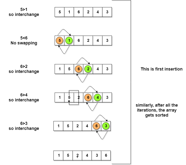
So as we can see in the representation above, after the first iteration, 6 is placed at the last index, which is the correct position for it.

Similarly, after the second iteration, 5 will be at the second last index, and so on.

Algorithm:

void bubbleSort(arr, n)
{
    int i, j, temp;
    for(i = 0; i < n; i++)
    {
        for(j = 0; j < n-i-1; j++)
        {
            if( arr[j] > arr[j+1])
            {
                temp = arr[j];
                arr[j] = arr[j+1];
                arr[j+1] = temp;
            } 
        }
    }
    
    return arr;
}

Hence the time complexity of Bubble Sort is O(n²).

What do you mean by optimization problem? Explain the greedy strategy for algorithm design to
solve optimization problems.

Explain the algorithm and its complexity for solving job sequencing with deadline problem using greedy strategy.

What do you mean by memorization strategy? Compare memorization with dynamic programing.

Memoization is a strategy to implicitly save the value of a computation in order to produce that same value later without evaluating the computation more than once.

Dynamic programming is a technique for solving problems of recursive nature, iteratively, and is applicable when the computations of the subproblems overlap.

Difference between Dynamic Programming and Memoization:

The difference between dynamic programming and memoization are

Dynamic Programming	Memoization
It is the research of finding an optimized plan for a problem by finding the best substructure of the problem for reusing the computation results.	It is the technique to “remember” the result of a computation and reuse it the next time instead of recomputing it, to save time.
It is a bottom-up approach.	It is a top-down approach.
Code gets complicated when left conditions are required.	Code is easy and less complicated.
It is fast, as we directly access previous states.	Slow due to a lot of recursion calls and return statements.
It is preferrable when the original; problem requires all subproblems to be solved.	It is preferable when the original problem requires only some subproblems to be solved.

Explain the concept of backtracking. How it differ with recursion?

Backtracking is a technique based on algorithm to solve problem. It uses recursive calling to find the solution by building a solution step by step increasing values with time. It removes the solutions that doesn’t give rise to the solution of the problem based on the constraints given to solve the problem.

Backtracking algorithm is applied to some specific types of problems,

• Decision problem used to find a feasible solution of the problem.
• Optimisation problem used to find the best solution that can be applied.
• Enumeration problem used to find the set of all feasible solutions of the problem.

In backtracking problem, the algorithm tries to find a sequence path to the solution which has some small checkpoints from where the problem can backtrack if no feasible solution is found for the problem.

Sl. No.	Recursion	Backtracking
1	Recursion does not always need backtracking	Backtracking always uses recursion to solve problems
2	A recursive function solves a particular problem by calling a copy of itself and solving smaller subproblems of the original problems.	Backtracking at every step eliminates those choices that cannot give us the solution and proceeds to those choices that have the potential of taking us to the solution.
3	Recursion is a part of backtracking itself and it is simpler to write.	Backtracking is comparatively complex to implement.
4	Applications of recursion are Tree and Graph Traversal, Towers of Hanoi, Divide and Conquer Algorithms, Merge Sort, Quick Sort, and Binary Search.	Application of Backtracking is N Queen problem, Rat in a Maze problem, Knight’s Tour Problem, Sudoku solver, and Graph coloring problems.

Explain in brief about the complexity classes P, NP and NP Complete.

P Class

The P in the P class stands for Polynomial Time. It is the collection of decision problems(problems with a “yes” or “no” answer) that can be solved by a deterministic machine in polynomial time.

Features:

1. The solution to P problems is easy to find.
2. P is often a class of computational problems that are solvable and tractable. Tractable means that the problems can be solved in theory as well as in practice. But the problems that can be solved in theory but not in practice are known as intractable.

NP Class

The NP in NP class stands for Non-deterministic Polynomial Time. It is the collection of decision problems that can be solved by a non-deterministic machine in polynomial time.

Features:

1. The solutions of the NP class are hard to find since they are being solved by a non-deterministic machine but the solutions are easy to verify.
2. Problems of NP can be verified by a Turing machine in polynomial time.

NP-complete class

A problem is NP-complete if it is both NP and NP-hard. NP-complete problems are the hard problems in NP.

Features:

1. NP-complete problems are special as any problem in NP class can be transformed or reduced into NP-complete problems in polynomial time.
2. If one could solve an NP-complete problem in polynomial time, then one could also solve any NP problem in polynomial time.

Write short notes on:
a. NP Hard Problems and NP Completeness
b. Problem Reduction

NP-hard class

An NP-hard problem is at least as hard as the hardest problem in NP and it is the class of the problems such that every problem in NP reduces to NP-hard.

Features:

1. All NP-hard problems are not in NP.
2. It takes a long time to check them. This means if a solution for an NP-hard problem is given then it takes a long time to check whether it is right or not.
3. A problem A is in NP-hard if, for every problem L in NP, there exists a polynomial-time reduction from L to A.

Some of the examples of problems in Np-hard are:

1. Halting problem.
2. Qualified Boolean formulas.
3. No Hamiltonian cycle.

NP-complete class

A problem is NP-complete if it is both NP and NP-hard. NP-complete problems are the hard problems in NP.

Features:

1. NP-complete problems are special as any problem in NP class can be transformed or reduced into NP-complete problems in polynomial time.
2. If one could solve an NP-complete problem in polynomial time, then one could also solve any NP problem in polynomial time.

Some example problems include:

1. Decision version of 0/1 Knapsack.
2. Hamiltonian Cycle.
3. Satisfiability.
4. Vertex cover.

b)Problem Reduction

We already know about the divide and conquer strategy, a solution to a problem can be obtained by decomposing it into smaller sub-problems. Each of this sub-problem can then be solved to get its sub-solution. These sub-solutions can then be recombined to get a solution as a whole. That is called is Problem Reduction. This method generates arc which is called as AND arcs. One AND arc may point to any number of successor nodes, all of which must be solved for an arc to point to a solution.

 

 

 

 

Problem Reduction algorithm:

1. Initialize the graph to the starting node.

2. Loop until the starting node is labelled SOLVED or until its cost goes above FUTILITY:

(i) Traverse the graph, starting at the initial node and following the current best path and accumulate the set of nodes that are on that path and have not yet been expanded.

(ii) Pick one of these unexpanded nodes and expand it. If there are no successors, assign FUTILITY as the value of this node. Otherwise, add its successors to the graph and for each of them compute f'(n). If f'(n) of any node is O, mark that node as SOLVED.

(iii) Change the f'(n) estimate of the newly expanded node to reflect the new information provided by its successors. Propagate this change backwards through the graph. If any node contains a successor arc whose descendants are all solved, label the node itself as SOLVED.